War Cycles

Previously I have shown that the Strauss and Howe saeculum is aligned with Kondratiev price cycles before 1650. The Kondratiev cycle at this time was shown to be consistent with a lagged Malthusian population growth model. Table 1 presents these Kondratiev cycles in terms of its half-cycle or Kondratiev wave. Kondratiev waves are typically defined as alternating periods of high and low inflation rate, but in this case they are periods of alternating high and low price level. This is because the Malthusian model predicts alternating periods of feast and famine that should be associated with low and high price levels, respectively. In all but one case the expected correspondence between the theoretical cycle driver and price level was seen. Also shown in the figure is socioeconomic stress, defined as the frequency of social unrest divided by the frequency of construction starts for religious buildings. The former is a measure of social turmoil while the latter is an economic indicator (presumably, famine period should be associated with both high price level and low rate of construction starts, giving a large ratio between the two (high socioeconomic stress). Feast periods would show the reverse, a small ratio and low socioeconomic stress. With two exceptions, periods of feast or famine correlated with low or high socioeconomic stress, respectively.

Table 1. Pre-1650 long cycles showing the action of the Malthusian population model (data from Table 1 in population model)

Turning	Kondratiev wave	Driver	Price	Socioeconomic stress
--	1176-1202	Feast	Low	Low
--	1203-1230	Famine	High	High
--	1231-1254	Feast	Low	Low
--	1255-1282	Famine	High	Low
--	1283-1305	Feast	Low	High
--	1308-1328	Famine	High	High
--	1329-1352	Feast	Low	Low
--	1353-1381	Famine	High	High
--	1382-1405	Feast	Low	Low
--	1406-1435	Famine	High	High
1435-1459	1436-1459	Feast	High	Low
1460-1487	1460-1487	Famine	High	High
1488-1517	1488-1520	Feast	Low	Low
1518-1542	1521-1557	Famine	High	High
1543-1569	1558-1579	Feast	Low	Low
1570-1594	1580-1602	Famine	High	High
1595-1621	1603-1626	Feast	Low	Low
1622-1649	1627-1650	Famine	High	High

A long cycle in Anglo-American history which I call the PE cycle has been approximately aligned with the Straus and Howe saeculum since 1720. The paradigm model was developed to explain both cycles for the period since ca. 1820. This paper attempts to address the period between 1650 and 1820 that is not covered by either model.

The PE cycle was defined as a consensus between the Schlesinger political cycle and an economic cycle based on dates for financial crises. The political cycle begins with the American revolution, and the first financial crisis which had an impact on American politics was in 1772. Between 1774 and 1860 the PE cycle periods were fairly well aligned with Kondratiev waves, as were the corresponding Strauss and Howe turnings. The alignment between turnings and Kondratiev waves continued further back and the PE cycle was extended before 1774 to 1720 using the consensus dates from Goldstein¹ for these waves. Before 1720 the alignment ends and the PE cycle is considered to have begun them.

Table 2 adds the 1650 peak and 1689 trough (dating from Goldstein¹) to give a set of eight periods between 1650 and 1860 that correspond to Kondratiev waves, exactly before 1774 and approximately afterward. These periods were analyzed in terms of inflation rate, unrest frequency and war intensity. Statistically significant relations were seen with all three: upwaves are times of inflation, increased war and lower unrest; downwaves are the opposite. That is unrest was inversely correlated with price: high prices/inflation were good times with low levels of unrest. Before 1650 unrest was directly correlated with price: high prices/inflation were bad times with high levels of unrest. This shift in social and economic interactions implies that a new cycle mechanism had come into play after 1650.

Table 2. Socioeconomic dynamics of long cycles over 1650-1860

Turning*	PE period	Description	Unrest events	Inflation rate	War Deaths per 100K pop.
1649-1675	1651-1688 (A)	Recession	0.98	-0.8%	25.3
1675-1704	1689-1719 (I)	Prosperity	0.58	0.9%	71.9
1704-1727
1727-1746	1720-1746 (A)	Recession	1.38	0.2%	16.1
1746-1773	1747-1774 (I)	Prosperity	0.79	1.0%	43.8
1773-1794	1774-1792 (A)	Recession	1.00	1.0%	11.0
1794-1822	1793-1823 (I)	Prosperity	0.45	0.8%	66.3
1822-1844	1824-1842 (A)	Recession	1.96	-1.1%	2.2
1844-1860	1843-1859 (I)	Prosperity	0.43	1.5%	11.3
Average (n=4)				-0.16%	48.3
Average 1650 (n=4)			1.33	1.05%	13.7
	p <=		3.8%	3.7%	4.0%

*Social moment turnings (crises and awakenings) in bold

Numerous observers, including Kondratiev, noted an association between upwaves and concentrations of war. Figure 1 shows a plot of war intensity, defined as deaths in great power² wars per 100,000 population.¹ War intensity shows 50-year cycles from the late 16^th through early 20^th centuries (see Figure 1). Concentrations of war do tend to occur during upwaves, which is reflected in the average war intensities in Table 2. These concentrations of war can be characterized in terms of the largest war within it, which is called a peak war. This terminology reflects a rough correspondence between the peak wars and Kondratiev peaks. The peak wars relevant to America are the War of Spanish Secession (Queen Annes war), Seven Years War (French & Indian war), the War of 1812, the American Civil War and World War I.

Figure 2 shows a plot of British imports³ relative to their long term trend over the 18^th century. Since colonial America was a key supplier of these imports, this data can give some insight into economic trends in the colonies. Also shown is a plot of US real unskilled labor costs⁴ for the 1790-1860 period. Figure 2 shows downturns in trade over 1724-46 and 1775-1790 and a period of zero wage growth over 1824-46. Figure 3 shows a continuation of the labor cost trend over 1850-1940. Real per capita GDP⁵ relative to its long trend is also plotted as a second economic indicator. The period is broken into four eras: 1846-1893 when wages were rising and GDP growth was above trend; 1893-1915 when wages were flat and growth was below trend; 1915-1929 when wages were rising and growth was on trend; and 1929-1940, which corresponds to the Great Depression. Two of these eras, 1893-1915 and 1929-1940 define periods of long-term economic decline. These two eras roughly correspond to periods of rising/elevated unrest (Figure 3). Table 3 presents these five periods of economic decline along with the end of the preceding peak war. Shortly after the end of the peak war and before the start of the downturn were the beginnings of war debt reduction (austerity). Dates for this are given in Table 3. Finally, dates for major financial crises associated with turning points in the PE cycle are given.

Table 3. Clustering of cycle turning points, peak wars, peak debt, panic and depression.

Peak War	War end	Start of austerity	Downturn	Financial crisis	Consensus turning point	PE active period	Social moment turning
War of Spanish Secession	1713	1717	1724-1746	1720	1721	1720-1847	1727-1846
Seven Years War	1763	1765	1775-1790	1772	1771	1774-1892	1773-1894
War of 1812	1814	1819	1824-1846	1819	1821	1824-1842	1822-1844
Civil War	1865	1870	None	1873	1869	1860-1873	1860-1865
None	--	--	1893-1915	1893	1892	1896-1919	1886-1908
World War I	1918	1922	1929-1940	1929	1927	1930-1946	1929-1946

The sequence of events in four of the six entries in Table 3 are consistent with the following model. Fighting wars results in a substantial increase in government outlays, which acts as an economic stimulus, increasing economic output and the price level. Hence periods when wars are fought should show inflationary prosperity, which is reflected in low levels of unrest and inactive periods in the PE cycle. Spending for wars leads to growth in government debt. At some point after the wars have ended, the government will begin to pay down its war debt by running budget surpluses (austerity). Imposition of austerity produces a disinflationary economy prone to financial crisis and prolonged economic downturns. Eventually both happen, triggering rising unrest and the beginning of an active period in the PE cycle. This sequence of events typically takes about a decade. I call this mechanism the war model.

The model breaks down for the Civil war. The expected sequence of end of the peak war, start of austerity, and financial crisis occurred, but the downturn did not materialize. Although the Panic of 1873 triggered the longest recession in American history, it was followed by a very strong recovery. The entire postwar era saw a rising trend in real wages (Figure 3). Not surprisingly there was no significant rise in unrest for two decades after the war. The 1860s do correspond to an active period and crisis turning, but both of these began before the Civil War. In fact it was the war itself, not an economic downturn, that was the driver for the crisis. Furthermore, a period of economic downturn beginning with the panic of 1893 and which showed elevated level of unrest was identified (Table 3). This period also corresponds to an active era in the PE cycle and an awakening turning, but it has no peak war. Two successive failures of the war model indicate that sometime between the War of 1812 and the Civil War, the war mechanism was replaced by another. This new mechanism was the paradigm mechanism previously described.

Historical action of war-linked financial crisis in the generation of active periods and social moments

The population model was still valid at the 1650 Kondratiev peak, but by the next peak in 1720 the war model was applicable. The unusually long Kondratiev cycle between these two dates contained three turnings instead of the normal two: an unraveling turning over 1649-75, the Glorious Revolution Crisis over 1675-1704 and a high turning over 1704-1727. Key reforms enacted as a result of the Glorious Revolution were responsible for the appearance of the war mechanism.

The direct result of the revolution in 1688 was the installment of a new king, William III, who recognized Parliament as a co-equal partner with the monarchy. When William proposed war with France, Parliament duly declared war in May 1689. The Commons, which had been responsible for authorizing war supply since the 15th century, deliberately kept William underfunded, requiring frequent war spending authorizations by Parliament, which kept Parliament in session almost continuously.⁶

Parliament developed innovative new taxes which were actually paid because they were seen by the public as legitimate because they came from Parliament. This established a regular means for securing government income that could be adjusted to actual needs. Parliament established a Commission of Public Accounts in 1690 to monitor government expenditures by the Crown and began inserting appropriations in its revenue bills that directed how the money was to be spent.⁶

Through these provisions Parliament gained control over the government budget, which helped ensure the success of the new central bank created in 1694.⁶ Not only was there now public control over government finance, budgetary issues were now explicit, allowing proper analysis of government debt as an investment. This created a direct link between government finance and the London financial and commercial community. In 1698 John Castaing began to issue a list of stock and commodity prices called The Course of the Exchange and other things at Jonathans Coffee House. It is the earliest evidence of organized trading in marketable securities in London.⁷

These innovations, collectively called the Financial Revolution, created market mechanisms through which wars could directly affect financial markets, leading to price rises (bubbles) and declines (financial crisis). An excellent example of this is the South Sea bubble. The South Sea Company was formed in 1711 as Tory competitor for the Whig Bank of England.⁸ The company was granted a monopoly on all British trade with the Spanish colonies in South America (then called the south sea trade) in exchange for taking over and consolidating the national debt. Consolidation meant getting owners of pre-existing loans to exchange them for South Sea company stock that paid a dividend that was smaller than the interest payment on original loan, which saved the government money. Holders of the loans were willing to do this for two reasons: (1) the stock was a liquid asset and so carried a liquidity premium, and (2) the stock had a potential for capital gain that the existing debt did not. What the South Sea company did was convert government debt from an investment (asset purchased for the income it provides) into a speculation (assets purchased for their capital gains potential). This is analogous to the recent practice of converting conventional mortgage loans into tradable mortgage securities.

The outcome was similar to what happened three centuries later. After the company directors circulated false claims of success in the South Sea trade the stock took off.⁸ Speculative fires were stocked when the government endorsed the company proposal for addition debt conversion over that of the Bank of England.⁸ The rising price of company stock helped spur general interest in the stock market as did the internet bubble. By the middle of 1720 market was flooded with a remarkable range of new ventures (the Pets.com of their day). 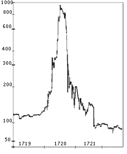Parliament passed the Bubble Act to outlaw the formation of these companies in an effort to prop up South Seas stock by minimizing competition for investor money. The stock peaked in early August and collapsed soon after (Figure 4). It continued to fall well into the next year, devastating institutions and individuals alike.⁸

Although historians have often assumed that this crisis, like later ones, had serious economic consequences, there is little statistical support for this.⁹ As shown in Figure 2, a downturn in trade volume relative to trend began years after the crisis. It did have serious political consequences, however, but these did not extend to America. This is not the case for the next war-linked financial crisis in 1772. Although the direct impact of the crisis was on the City of London, it exerted indirect effects that led to the American revolution as described by Schwarz:¹⁰

In the summer and fall of 1772, panic took hold of Londons financial circles. It began with the collapse of a firm called Neale, James, Fordyce, & Down. Alexander Fordyce had been speculating successfully for a decade, but in the early 1770s his investments went sour. He managed to deceive his partners for a while; according to one biographer, It is said he succeeded in quieting their fears by the simple expedient of showing them a pile of bank notes which he had borrowed for the purpose for a few hours. When things got too hot, though, Fordyce skipped town owing a hundred thousand pounds. In early June his firm suspended payment of its debts.

In a generally overextended market many other firms were just as vulnerable, and the dominoes started falling. By the end of June twenty major houses had collapsed. Those that were left suffered the usual squeeze: Debtors were slow to pay, while creditors were quick to demand payment. Among the hardest hit was the already foundering East India Company, which had a monopoly on trade, chiefly in tea, with the British Asian colonies.

In September the company took out a loan from the Bank of England, to be repaid from the sale of goods later that month. But with buyers scarce, most of the sale had to be postponed, and when the loan fell due, the company coffers were empty. On October 29 the bank refused to renew the loan. That decision set in motion a chain of events that made the American Revolution inevitable.

The East India Company had eighteen million pounds of tea sitting in British warehouses. Selling it in a hurry would do wonders for its finances. The American market beckoned, but there were two problems. First of all, the company was required by law to sell its tea to the highest bidder in England, letting merchants there and in America ship and resell it. Second, tea sold in America carried a tax of three pence a pound, which made it unpopular with restive colonists.

After prolonged wrangling, in May 1773 Parliament let the company eliminate the middleman and market the tea itself through its own American agents. It also refunded duties that the company had paid upon bringing the tea to England. With these changes the East India Company could easily undercut the smugglers who had been taking much of its business. On the tax issue, however, the government would not budge. While admitting that three pence a pound yielded negligible revenue, it insisted on maintaining British taxation power over its colonies.

It seemed a perfect compromise: The company would make money, the colonies would get cheap tea, and Britain would uphold its rights. So the government was quite surprised when citizens in Charleston, Philadelphia, New York, and most famously Boston vigorously rejected the tainted tea. Their tea parties showed that America would not be bribed into accepting taxation without representation. Yet that was not the only issue.

There was nothing new about the tea tax. Colonists had been paying it--and similar taxes on sugar, molasses and win--for years. The new and obnoxious feature of the Tea Act was the monopoly for the East India Company, which would deprive American merchants of their business in both legal and smuggled tea (and which they feared would be extended to many other goods). By alienating this wealthy and powerful group, the British united self-interest and revolutionary fervor in a combination that would soon destroy the colonial bond. Just as the failure of a single bank had caused a financial panic, so too did a seemingly innocuous attempt to collect a tax that was already on the books lead directly to the American Revolution.

Within two years of the tea parties, armed rebellion had broken out, which expanded to full-scale war by the next year. The outbreak in hostilities led to the downturn in trade that began in 1775. So the crisis of 1772 led to both political and economic changes consistent with the start of an active period or social moment turning and can be considered as a triggering event for both.

The role of the Panic of 1819 in the rise of Jacksonian populism that characterized the 1824-1842 active period in the PE cycle was previously discussed. This crisis ended the Era of Good Feelings by accentuating political division over the role of the central bank in the panic. In time these divisions became formalized in the establishment of the Democratic and Whig parties, and the rise of the paradigm mechanism. Here the war-induced financial crisis gave rise not only to economic stress and its associated unrest, but also to political forces that produced a liberal era and the paradigm derived from it.

As described earlier, the next war-linked financial crisis, the Panic of 1873, did not play a role in initiating a social moment turning or active period for a crisis turning and active period in the PE cycle. Financial crisis continued to be a factor in producing active eras/social moment turnings after 1873. In fact, in three of the four active eras/social moment turnings after the Civil War, financial crises (in 1893, 1929 & 2008) played important roles. Since 1720, only two of the eight active eras/social moments have not involved economics as a dominant factor. Both of these (Civil War and Civil rights era) had triggering events associated with an overriding social issue (race relations).

The genesis of the modern politically-driven cycles (war and paradigm) was the financial revolution associated with the Glorious revolution. Strauss and Howes generational cycle characterizes this period as secular crisis, a period that addresses the outer world of institutions, as opposed to the spiritual awakening, which addresses the inner world of private belief and behavior. Social moments correspond to active eras in the PE cycle, but the PE cycle methods do not apply to this time, nor do the social dynamics support a Glorious Revolution social moment, (unrest was not particular high at this time). This period occurs outside of the scope of my empirical cycle methods, although it is undeniably a crisis era in the sense that Strauss and Howe use. It is only after this crisis that the patterns characterizing the PE cycle became valid.

From the very beginnings of financial markets in the wake of the Glorious Revolution, finance has been intertwined with politics, with the latter in the drivers seat. Initially, it was war policy by the monarch that was the driver. Quincy Wright, who was first to characterize the war cycle, proposed a number of factors as possible causes for periodicity of war. One factor were alternating hawk and dove generations: The warrior does not wish to fight again himself and prejudices his son against war, but the grandsons are taught to think of war as romantic.¹² The financial impact of these cyclical wars produces cyclical unrest that defines the PE and turning cycles. With the rise of mass democracy, I have proposed dominant and recessive paradigmic generations to replace hawk and dove generations, but it is still the impact of politics on policy affecting the economy and society that gives rise to active eras and social moments. For example the recent financial crisis was made possible by decades of supply side economic policy introduced as part of the Freedom paradigm established during the 1966-1981 active era. Since then, high interest rates, as opposed to high taxes, have been the preferred means to control inflation, which penalizes capital-intensive industries like manufacturing, to the benefit of finance. Preferential tax treatment of capital gains over income encourages speculation as opposed to investment, much as did government sponsorship of the South Sea company.

Development of the War Cycle

As Figure 1 shows, there is some evidence for the cycle existing as early as the late 16^th century, and certainly during the first half of the 17^th century. Early 16^th century wars showed no evidence of cycles (see Figure 5). Interactions between war finance and the Kondratiev cycle can explain the rise of the war cycle. Wright proposed that financial constraints force temporary cessations of war expenditure to give the economy time to recovery: there is a tendency to postpone a new war until there has been time to recover economically from the last.¹³

The scale of warfare had grown tremendously during the 16th and early 17th centuries culminating in the cataclysm of the Thirty Years War, a phenomenon called the Military revolution. This growth placed a severe strain on the ability of nations to pay for the wars they fought. Spain was the only belligerent involved in all these major wars and for whom the problem of payment was most acute, Despite the steadily increasing stream of silver and gold from their American colonies, Spain underwent no less than seven state bankruptcies over the 1500-1650 period.^14,15 Most of these bankruptcies came from excessive war-spending. The bankruptcies of 1557 and 1607 more or less forced the Treaty of Cateau-Cambresis in 1559 and the truce of 1609 which established the de facto independence of the Netherlands from Spain. Spain never learned to reign in her ambitions and when the growth in flow of American treasure slowed in the 1630s, she began a permanent decline that ended her days as a great power by the end of the century. As the Spanish captains used to say, victory went to him who has the last escudo.¹⁵

The example of Spain could serve as an object lesson in the problems that came from ignoring finance. The other European powers had the luxury of not always being involved in conflict, and so were better able to time their war-fighting so as to avoid fiscal catastrophe. The population-derived Kondratiev cycle created alternating periods of higher or lower inflation. The former were good times to incur debt since it could be repaid using less valuable currency. Hence there was a natural tendency for wars of choice to cluster during upwaves, giving rise to a war cycle aligned with the Kondratiev cycle as depicted in Figures 1 and 4. That is, price cycles of feast/famine(and the associated good/ bad times) induced cycles of peace/war, which, as the financial revolution unfolded, induced cycles of depression/prosperity (associated with bad/good times). That is, around the time of the Glorious revolution, the alignment between unrest and price shifted from inflation being bad (famine) to inflation being good (prosperity). Such a shift would necessarily affect the alignment between Kondratiev cycles and the saeculum. The 1650-1843 period contains 3.5 Kondratiev cycles of 55 years, implying a saeculum length of 110 years at the normal ratio of two Kondratievs per saeculum. The shift in alignment caused by the financial revolution forced the addition of one extra turning in order to avoid sequential social moments. This means that two saecula fell into the 1650-1843 period containing only 3.5 instead of 4 Kondratievs. This implies a shortening of the saeculum length from 110 to 96 years. The actual average saeculum length for the two saecula before 1649 was 107 years, compared to 94 years for the two after.

Summary

This graphic summarizes the various long cycles I have described in terms of when they were operative The first four rows describe an economic cycle, a generational cycle, a political and economic cycle, and a war cycle. The next two rows show when the three models I have presented were operational. Overlapping the beginning of each model is the revolution that made the mechanism possible. The military revolution created the need for finance, which led to the war cycle. The financial system created to manage wars during the financial revolution spawned the war cycle, which after the democratic revolution was replaced by the paradigm mechanism.

12^th cent

13^th cent

14^th cent

15^th cent.

16^th cent.

17^th cent.

18^th cent

19^th cent

20^th & 21^st cent

50-year Kondratiev cycles

Long K-cycle

Century-long saeculum

Variable length saeculum

PE cycle

War Cycle

Malthusian Model

Paradigm model

War model

Revolutions:

Military

Financial

Democratic

References

1. Goldstein, Joshua S. Long Cycles, New Haven: Yale University Press, 1988

2. In 1650 the great powers were the Austrian empire, Britain, France, the Netherlands, the Ottoman empire, Prussia/Germany, Spain and Sweden. Sweden, the Netherlands and the Ottomans are dropped after 1715 while Russia is added. Spain drops out after 1800; the United States and Italy are added after 1850.

3. British import volume is the official value (in British pounds) of imports. It was obtained from Mitchell (ref 13) for the period 1700-1853. A second series of computed values is given for 1796-1853. The ratio of the computed values to the official value shows a shape similar to the price index over the 1796-1853 period. If the computed values are divided by a price index to put them in real terms the resultant series is very similar to the official series. Thus, the official trade statistics appear to be a proxy for trade volume in real terms and so were used directly for analysis.

4. Lawrence H. Officer and Samuel H. Williamson, Annual Wages in the United States, 1774-Present, MeasuringWorth, 2014.

5. Samuel H. Williamson, What Was the U.S. GDP Then? MeasuringWorth, 2014.

6. parliament.uk, The Financial Revolution, Living Heritage The Glorious Revolution

7. London Stock Exchange Our History

8. Harvard Business School, South sea bubble short history

9. Hoppit, J. (2002) The Myths of the South Sea Bubble, Transactions of the Royal Historical Society, 12: 141-165.

10. Frederic D. Schwarz, 1772: two Hundred And Twenty-five Years Ago, American Heritage, 48(6), October 1997.

11. Cycles in American History

12. Wright, Quincy, A Study of War, 1942; reprint ed. Chicago: University of Chicago Press, 1965, p 230.

13. Ibid p 1272

14. Richard Cavendish, Spanish Bankruptcy, History Today

15. Spain then and now; 16th C Spain. Overview: Politics.

16. Kennedy, Paul, The Rise and Fall of the Great Powers, New York: Vintage Book, 1987, p xxiv.

17. Mitchell, B. R. British Historical Statistics, Cambridge University Press, 1988.